
Metrics for vulnerability prioritization for Microsoft products - A data science mini project
Summary
I set out to find out if publicly available data could provide additional or, better yet, stronger indicators for vulnerability prioritization than the de facto standard of CVSS score.
To limit the scope of my initial project in this field, I chose to focus on Microsoft as the dominant vendor and used only vulnerabilities published in 2020 and 2021.
For Microsoft products I was able to find additional data that can help in prioritization. Namely Microsoft’s own assessment of likelihood of exploitation, the product category, and mentions in CISA and NCSC-FI bulletins.
My findings summarized:
- Primary indicator is Microsoft’s own likelihood of exploitation
- Secondary indicator is the affected product
Caveat:
- It is worth noting that vulnerabilities’ status changes over time were not taken into account, i.e. vulnerabilities that were immediately exploited now rank the same as vulnerabilities that were exploited later on => both are “Exploitation detected”.
Background
I am interested in the topic of vulnerability management from a professional setting. I work for the National Cyber Security Centre of Finland and have previously worked as a CERT team member and now I am heading a unit which focuses on enabling the CERT and situational awareness functions to operate more efficiently.
Analyzing the monthly cycle of updates is a big part of the CERT team’s efforts to help organizations focus on the right things to prioritize limited IT resources on.
Previously NCSC-FI has released an article on the arms race of patch management vs exploit development which painted a fairly dire picture of the situation.
With this project I wanted to dig a bit deeper and see if I could find other distinguishing features for more dangerous, or to be more specific, exploits that are more likely to be exploited than others.
This is meant to provide assistance to both CERT team members doing the initial evaluation of disclosed vulnerabilities as well as the IT and cyber security professionals responsible for the actual patching at different organizations.
The status quo and the null hypothesis is that CVSS score is the defining feature of vulnerability prioritization.
Step 1: Identify, collect and explore data
My originally identified data sources were:
- CVEDetails.com
- CVE.org
- Mitre CVE db
- Nist NVD
- NCSC-FI News and vulnerabilities digests
- NCSC-FI Vulnerability Alerts
- CISA Catalogue of known exploited vulnerabilities
- Exploit-db
The data I was collecting fell into three categories:
- Basic metadata
- CVE number (i.e. the main identifier)
- Vendor and product
- Description
- CVSS score (1.0 - 10.0 scale from Low to Critical)
- Additional features
- Mentions in reputable expert publications
- Severity of alerts
- Proof of exploitation/exploitability
- Number of exploits found in different sources
Collection and wrangling of data was fairly straight-forward to begin with. CVEDetails provides an option to download the vulnerabilities as tables of tab-separated values (.tsv) and I could read these into pandas in the Jupyter Notebook I was using as my interactive documentation throughout the investigation.
The total sum of CVEs to start me off was 1220 and 909 for the two years for a total of 2129 CVEs.
CVE.org and Mitre did not provide additional details, but Nist NVD provided a breakdown of ‘CVSS Score’ to its constituent components and both v2 and v3 of the score.
<Sidenote on CVSS>
CVSS score is made up of several features.
For example a vulnerability with this set of features and values:
- Attack Vector (AV): Local
- Attack Complexity (AC): Low
- Privileges Required (PR): Low
- User Interaction (UI): None
- Scope (S): Unchanged
- Confidentiality (C): High
- Integrity (I): High
- Availability (A): High
Can be displayed in shorthand CVSS:3.1/AV:L/AC:L/PR:L/UI:N/S:U/C:H/I:H/A:H which is set next to the total score, impact score and exploitation score.
</Sidenote on CVSS>
NCSC-FI news and vulnerability digests I gathered from my personal email archives, removed email headers, and did some other simple text cleaning.
Hurdle no. 1
How do I actually verify that specific vulnerability is or has been actively exploited?
CVEDetails.com has a data field called # of Exploits but for all vulnerabilities published in 2020-2021 this field was empty! This was the first issue I discovered by looking at the data.
I was stuck on this for quite some time as I soon discovered that Exploit-db yielded zero results with its searchsploit tool when I iterated through the ~2000 CVEs.
I believe one of the reasons Exploit-db did not yield results is that exploit writers might be less interested in tagging the correct CVE number and more interested in using fancy branded vulnerability names like PrintNightmare (CVE-2021-1675 & CVE-2021-34527) or ZeroLogon (CVE-2020-1472). This would warrant further linking of names to CVEs in future projects.
The initial stand-in variable was a combination of whether CISA’s catalogue of known exploited vulns contained the CVE or if the NCSC-FI vulnerability digest had indicated Exploitation as PoC, Yes or Wild.
At this point the data set had only 12 out of 2129 (0,5%) vulnerabilities can be determined to be exploitable. That is a massively unbalanced set of data.
Looking at the data I noticed that NCSC-FI alert feed, a fairly strong indicator of importance, had very few mentions of actual CVE numbers. This prompted me to go fetch the HTML content of the linked alert pages and find CVE numbers therein.
This increased the number of potentially dangerous CVEs from 12 to 55. A good start, but still too unbalanced.
It was at this point that I was still aware of the large unbalance and was not very hopeful for a good outcome. This split of exploited/not exploited data was strongly indicating that CVSS score was the dominant factor as I did some very simple tests with regression models.
When I contacted someone with more expertise, they recommended different approaches to over- and undersampling and mentioned a specific technique called SMOTE for which I did find a good article on but failed to get it to work as I had not yet mastered one-hot encoding for categorical data.
I put that aside as something to look into but continued to try and find some other data that could be of more use.
Then I looked at what data e.g. Microsoft’s own website provides and there I noticed an interesting table with data:
| Publicly disclosed | Exploited | Latest software release |
|---|---|---|
| Yes | No | Exploitation Less Likely |
Eureka! I had finally found some clearly defined category for deciding if a specific vulnerability is/was exploited.
Quick stats told me:
| Count | Exploited |
|---|---|
| 2036 | No |
| 28 | Yes |
| Count | Exploitation category |
|---|---|
| 26 | Exploitation Detected |
| 1840 | Exploitation Less Likely |
| 155 | Exploitation More Likely |
| 3 | Exploitation Unlikely |
| 25 | N/A |
| 57 | null |
I was far too excited with the discovery of these four categories that I did not do the math on the distribution of these classes at the time. This would end up biting me in the ankle later on.
This covered the gap made by zero results from CVE Details’ number of exploits feature and zero results from exploit-db. This category allowed me to avoid using other features to create a synthetic label.
Looking at the data now showed that the additional features of NCSC-FI vulnerability alerting and CISA known exploit actually produced three different categories of Microsoft assessments.
| # | MS Category |
|---|---|
| 34 | Exploitation Less Likely |
| 27 | Exploitation More Likely |
| 27 | Exploitation Detected |
Here again, the categories look all nice and even. Except the query did not return majority class which was two orders of magnitude bigger than any of these smaller ones.
Step 2: Visual EDA
I had finally wrangled, coaxed, merged and cleaned data to a master dataframe in pandas.
A single row looked something like this:
| 0 | |
|---|---|
| cve | CVE-2020-26870 |
| CWE | 79 |
| Vuln type | XSS |
| Published | 2020-10-07 00:00:00 |
| Updated | 2021-07-20 00:00:00 |
| Score | 4.3 |
| Description | Cure53 DOMPurify before 2.0.17 allows mutation XSS. .. |
| score_v2 | 4.3 |
| exploitability_v2 | 8.6 |
| impact_v2 | 2.9 |
| score_v3 | 6.1 |
| exploitability_v3 | 2.8 |
| impact_v3 | 2.7 |
| cisa_exploitable | 0 |
| ncscfi_alert | 0 |
| vulns_mention | 0 |
| news_mention | 0 |
| ncscfi_exploit_rank | 0 |
| product | Visual Studio |
| public | 0 |
| latest_rank | 0.33 |
| older_rank | 0.33 |
| exploitation_rank | 0.33 |
| exploitation_category | Exploitation Less Likely |
| exploitation_confirmed | 0 |
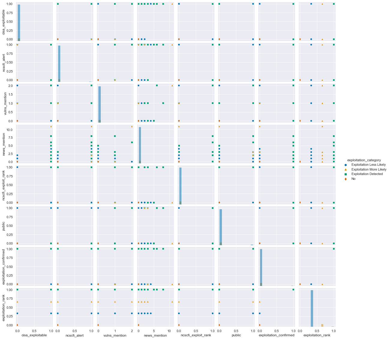
I followed along simple lines and did a seaborn pairplot to see if any correlations and potential patterns could be found.
g = sns.pairplot(build_cve(), hue='exploitation_category', height=2, palette='colorblind', markers=['o','^', 's', 'd'])
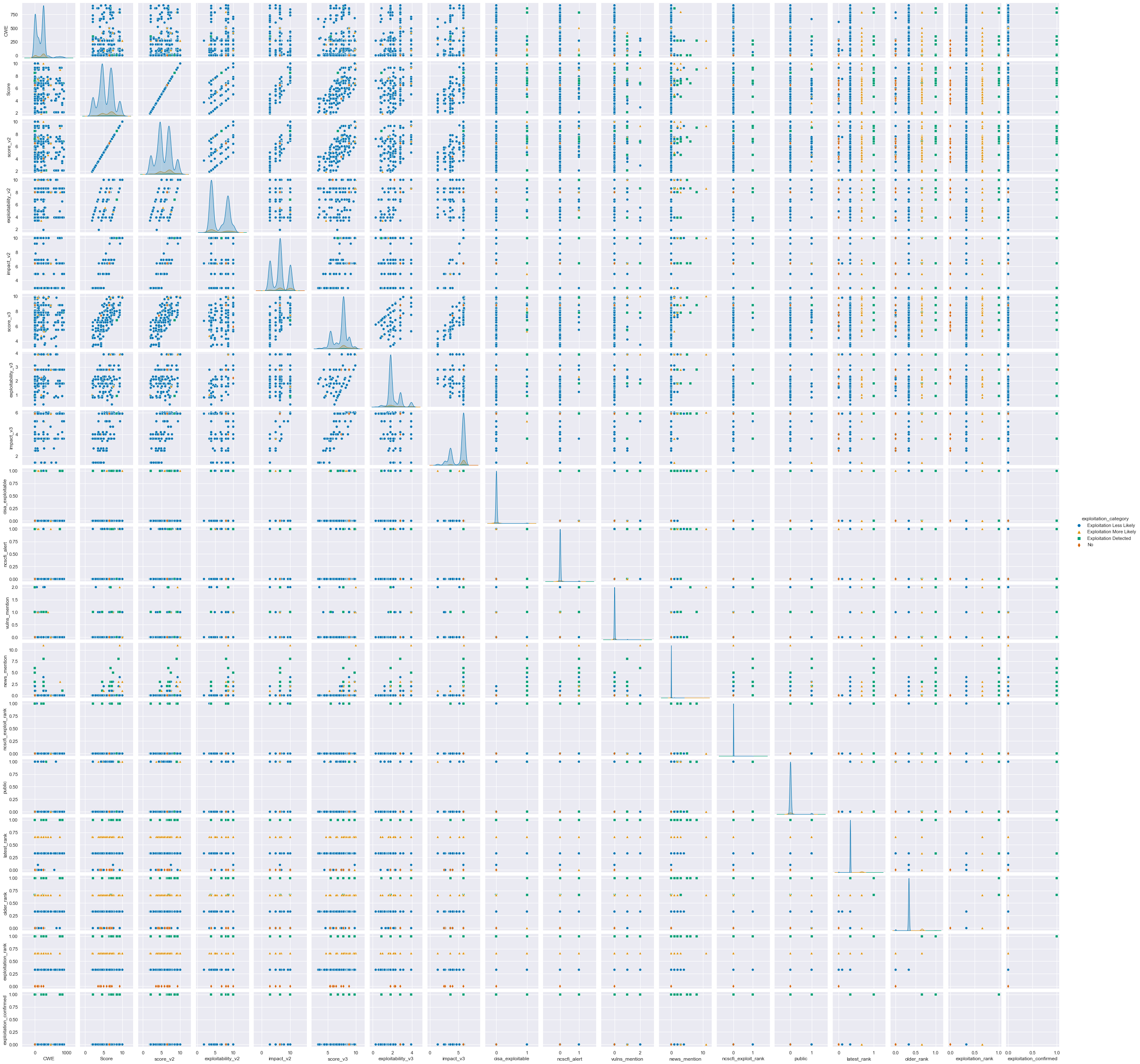
There are some clear direct linear relations between the fields and that is not surprising, since the first fields are mostly CVSS scores or their subcomponents which are by definition tied together.
The second thing I noticed was that all of the rest of the data is very sparse and more categorical. Things have either been mentioned in the news once or they haven’t etc.
This meant that I would probably be better served with a logistic regression for multi-class classification instead of a linear one for continuous data.
Step 3: Principal component analysis
For this step I had a brilliant source to follow closely: Python Data Science Handbook - 05.09 Principal Component Analysis.
I had built myself some helper functions to be able to start my analysis, model fitting etc. tasks in each Jupyter Notebook cell from a clean slate.
# src: https://jakevdp.github.io/PythonDataScienceHandbook/05.09-principal-component-analysis.html
from sklearn.decomposition import PCA

cve = build_cve()
X, y = make_X_y(quantified_fields(cve))
display(X.shape) # (2062, 12)
pca = PCA()
pca.fit(X)

plt.plot(np.cumsum(pca.explained_variance_ratio_))
plt.xlabel('number of components')
plt.ylabel('cumulative explained variance');
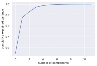
And the curve looked similar to the examples in the handbook - quick rise and then it has diminishing returns. But amazing - I would get more than 90% of all data variance from two features alone! That will make my model fitting super easy.
This turned out to be false of three different reasons: the data was unbalanced, I only had columns as continuous numbers and not as classes, and I still had CVSS subcomponents in the feature list which was the exact opposite of what I was originally looking for. But this discovery happened after a week of testing different models and fits and permutations of features.
Step 4: Model fitting and scoring
Logistic regression
Using LogisticRegression from sklearn.linear_model I was able to achieve excellent results from the beginning - in the ballpark of 90% accuracy over my 2 year data set. The only thing I needed to fine-tune was the max_iter parameter to a higher number.
| Predictions | |
|---|---|
| P(Exploitation Detected) | 0.1% |
| P(Exploitation Less Likely) | 96.0% |
| P(Exploitation More Likely) | 1.8% |
| P(No) | 2.2% |
| Accuracy over data set | 91.0% |
Since the PCA was so promising, I tried how well it would fit the data predictions:
| 0 | |
|---|---|
| P(Exploitation Detected) | 0.6% |
| P(Exploitation Less Likely) | 94.3% |
| P(Exploitation More Likely) | 3.4% |
| P(No) | 1.7% |
| Accuracy over data set | 90.1% |
Amazing results - I was very excited about this prospect and even more so about actually getting the models to work as they did in the examples and documentation!
I then tried some RepeatedStratifiedKFold splits to vary features across model fits.
def fit_model(X_train, X_test, y_train, y_test):
    model = LogisticRegression(max_iter=1500)
    model.fit(X_train, y_train)
    result = model.score(X_test, y_test)
    print("Accuracy on test set: %.2f%%" % (result*100.0))

folds = RepeatedStratifiedKFold(n_splits=10, n_repeats=3, random_state=42).split(X, y)
for train_index, test_index in folds:
    X_train, X_test = X.iloc[train_index], X.iloc[test_index]
    y_train, y_test = y.iloc[train_index], y.iloc[test_index]
    fit_model(X_train, X_test, y_train, y_test)
And again great results but at least with some variation to (falsely) give me verification that this was good model and it sometimes even went below 90% accuracy.
Accuracy on test set: 91.04%
Accuracy on test set: 89.59%
Accuracy on test set: 90.53%
Accuracy on test set: 90.78%
Accuracy on test set: 90.29%
I even did cross validation:
model = LogisticRegression(max_iter=10000)
scoring = 'accuracy'
results = model_selection.cross_val_score(model, X, y, scoring=scoring)
print('Accuracy on validation set: %.2f%% (std = %.2f)' % (results.mean()*100, results.std()))

# Accuracy on validation set: 90.93% (std = 0.01)
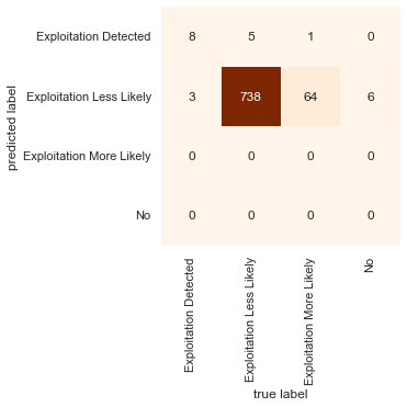
The confusion matrix of predicted labels vs true labels:
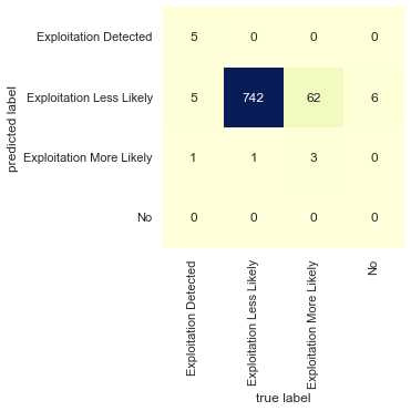
Random forest classifier
According to material I had used to learn the basics of data science, random forest classifiers are quite superb out-of-the-box algorithms for classification. I did not know how much better my results could get since the simple logistic regression was already at 90%.
Giving it a go produced similar accuracy as before:
# This time I wanted to see if only non-cvss features could yield good results
X = cve[['cisa_exploitable', 'ncscfi_alert', 'vulns_mention',
         'news_mention', 'ncscfi_exploit_rank', 'public',]]
y = cve[['exploitation_category']]

X_train, X_test, y_train, y_test = train_test_split(X, y, stratify=y, test_size=0.40, random_state=1)

rfc = RandomForestClassifier(max_depth=2, random_state=5)
rfc.fit(X_train, y_train.values.ravel())

print(rfc.score(X_test, y_test)) # => 0.9042424242424243

predictions = rfc.predict(X_test)
mat = confusion_matrix(y_test, predictions)
sns.heatmap(mat.T, cmap="Oranges", square=True, annot=True, fmt='d', cbar=False,
            xticklabels=rfc.classes_, yticklabels=rfc.classes_)
plt.xlabel('true label')
plt.ylabel('predicted label');
Now that I had the model set up, I started manually varying the chosen features just to derive some insight as to which were the most important. I wanted to go even further away from CVSS scores so I wanted to take the description of the vulnerabilities and see if it could be used to predict vulnerability class - similar to Python Data Science Handbook > Multinomial Naive Bayes example.
OneHotEncoder
In order to take the product name and vulnerability descriptions as my features, I would have to quantify them because I was stuck with the error message ValueError: could not convert string to float: 'Windows Event Tracing'.
My materials and StackOverflow pointed me to OneHotEncoder from sklearn a solution.
This goes through all the possible values of a given categorical field and explodes all potential values as colums “type_A”, “type_B” etc.
For example the product field yielded 239 columns from the 2062 rows and description yielded 1820 differing values.
The simplest form was
from sklearn.preprocessing import OneHotEncoder
onehot = OneHotEncoder(handle_unknown='ignore', sparse=False)
X_hot = pd.DataFrame(onehot.fit_transform(X))
This allowed me to see how well e.g. product or description feature would fare.
Using OneHotEncoder and product gave me 90% accuracy.
Look at the data! I found that one of the one-hot columns was always 0 - at one point in my refactoring of code, I had inject a logic failure. Verify your assumptions!
Cool! Maybe I could find if some specific products like Windows Kernel or Print Drivers would be a bigger indicator for exploitability.
I googled sklearn model coefficient to understand how to represent the calculated model and weights. I stumbled upon this article Common pitfalls in the interpretation of coefficients of linear models. Some of the math was a bit hard to get my mind around, but I was able to do a similar result on the product field.
To simplify my results, I turned my multi-class into binary classification with
cve.loc[cve.exploitation_rank > 0.5, ['ms_exploitation_combo']] = 'More Dangerous'
cve.loc[cve.exploitation_rank < 0.5, ['ms_exploitation_combo']] = 'Less Dangerous'
The top and bottom 5 coefficients in my data set
| Coeff | |
|---|---|
| product_Windows Common Log File System Driver | 2.84966 |
| product_Windows TCP/IP | 2.18728 |
| product_Windows Win32K | 2.11566 |
| cisa_exploitable_1 | 1.8105 |
| product_Microsoft Graphics Component | 1.64057 |
| product_Windows Kernel | 1.63954 |
| .. | .. |
| product_Microsoft Office | -0.697544 |
| product_Microsoft JET Database Engine | -0.785466 |
| product_Visual Studio | -0.818753 |
| product_Microsoft Windows Codecs Library | -0.92459 |
| product_Azure Open Management Infrastructure | -1.09634 |
So my initial finding is that if the Windows products Win32K, TCP/IP or log driver are mentioned, they strongly indicate more danger and Microsoft Azure on the other hand should lessen your blood pressure. (Note: There were multiple products with ‘office’ in the name, this wasn’t the only row)
It seemed like I had found an answer to the question: are there other features besides CVSS score that could be used to prioritize?
But then I tried using OneHotEncoder and description and it also produced 90% accuracy even though a better fit probably would have been TfidfVectorizer + MultinomialNB.
…
It was a this point I went hmmmmmmmm.
Step 5: When random is 90% correct
A rabbit hole, a red herring, a diversion, a distraction.
At first I started backtracing my steps and it just got very confusing very fast - so I started from the top and went step by step.
Then I realized my mistake which I aluded to earlier. The data was still heavily skewed even if there were numerically more categories - they still weren’t being filled uniformly.
The model was predicting everything to be less dangerous, less exploitable since it was the best guess.
Adding a very crucial column to this table aids in seeing the problem
| Predictions | Actual distribution | |
|---|---|---|
| P(Exploitation Detected) | 0.1% | 1.3579 |
| P(Exploitation Less Likely) | 96.0% | 90.1067 |
| P(Exploitation More Likely) | 1.8% | 7.80795 |
| P(No) | 2.2% | 0.727449 |
| Accuracy over data set | 91.0% | 100 |
If the distribution is not uniform, but this heavily biased, then guessing the majority class for all items will produce 90% accuracy. To get an actual estimate of accuracy, the data would need to be more evenly distributed and that means either reducing the majority class (undersampling) to be in the same magnitude as the minority ones or by some means increase the population of the minority ones (oversampling).
Step 6: SMOTE
I then returned to the advice I had already been given before I got too excited with multi-class labeling from Microsoft. SMOTE, or Synthetic Minority Oversampling Technique, seemed like a good idea since I would rather have more data than less.
First smotin’
from imblearn.over_sampling import SMOTE
X, y = make_X_y(qdata)
oversample = SMOTE()
Xo, yo = oversample.fit_resample(X, y)
clf = LogisticRegression(random_state=0, max_iter=1500).fit(Xo, yo)
print("Accuracy {:.1%}".format(clf.score(Xo, yo)))
Now that the data set’s distribution for the four classes was 25:25:25:25 I was able to get a more moderate result:
| Accuracy over data set | Features |
|---|---|
| 68% | Logistic regression with all numeric / non-categorical fields |
| 68% | Same as above, but with RepeatedStratifiedKFold |
| 33% | Logistic regression with PCA reduction to 1-dimensional feature set |
| 60% | Logistic regression with non-CVSS fields |
All of these were previously >90% due to data distribution.
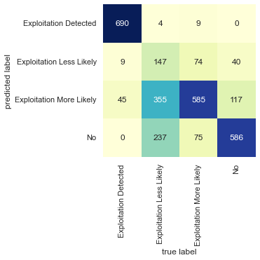
Much more confusion in the predictions.
The article gave a fairly good walk-through on how to get a simple SMOTE oversampling going on with my data set. It pointed out that a combination of over- and undersampling would perhaps be even better:
The original paper on SMOTE suggested combining SMOTE with random undersampling of the majority class.
So the following data models and fittings were done with this pipeline:
from imblearn.over_sampling import SMOTE
from imblearn.under_sampling import RandomUnderSampler
from imblearn.pipeline import Pipeline

over = SMOTE()
under = RandomUnderSampler()
steps = [('o', over), ('u', under)]
smote_pipe = Pipeline(steps=steps)
# Potential OneHotEncoder here
X, y = smote_pipe.fit_resample(X, y)
Repeat model fitting, scoring, tuning
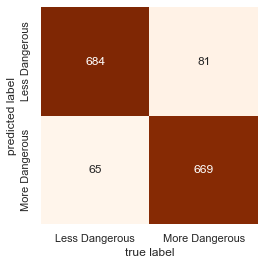
Given that the logistic regression was performing fairly poorly it was actually on par to what I expected to begin with.
Some RandomForestClassifier accuracy statistics with different feature sets:
| Accuracy | Description |
|---|---|
| 58% | CVSSv2 Score |
| 50% | CVSSv3 Score |
| 82% | Non-CVSS fields (CISA, NCSC-FI mentions) |
| 54% | Non-CVSS fields no product |
| 80% | Only product |
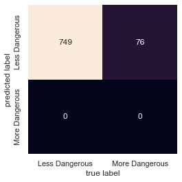
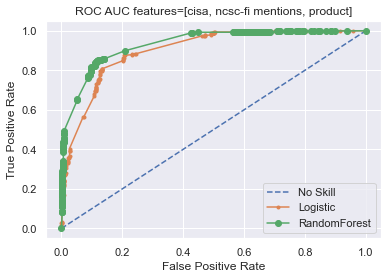
ROC AUC
The same post about SMOTE also taught me about “ROC area under curve (AUC) metric” which sounded like potentially interesting metric and provided example code to actually calculate it.
I used the two classifier models (LogisticRegression and RandomForestClassifier) with a binary model based on Microsoft’s Less/More likely
ex_rank = {
    'No': 0.0,
    'Exploitation Unlikely': 0.1,
    'Exploitation Less Likely': 0.33,
    'Exploitation More Likely': 0.66,
    'Exploitation Detected': 1.0
}

y = cve['exploitation_rank'].map(lambda val: 1 if val > 0.5 else 0)
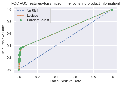
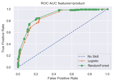
ROC AUC Results
| No skill | Logistic | Random Forest | Features |
|---|---|---|---|
| 0.500 | 0.902 | 0.927 | CISA, NCSC-FI mentions, product information |
| 0.500 | 0.671 | 0.674 | CISA, NCSC-FI mentions, no product information |
| 0.500 | 0.872 | 0.894 | only product information |
Step 7: Results
My findings summarized:
- Primary indicator is Microsoft’s own likelihood of exploitation
- Secondary indicator is the affected product
Microsoft’s likelihood of exploitation
An overlooked data source for vulnerability prioritization is Microsoft’s own assessment of the probability of exploitation.
![]()
As can be seen, the distribution of both versions of CVSS scores is not particularly focused on any one Microsoft exploitation likelihood category, which I chose as the best available ranking of exploitability.
Microsoft product name
As the secondary indicator the model would give weight to product - which is curious since the list of product names is varied to say the least. There is much more data transformation that could be done with this list of 285 different product names, but it would require more ontological decisions and digging through the 2000 vulnerabilities’ details than my schedule now permits.
For example should Azure and Azure SDK be combined? But what about Azure AD Web Sign-in and Azure Active Directory Pod Identity – the Azure AD stuff is surely different from a generic SDK vulnerability, but whether these two Azure AD product names are related and groupable - I don’t know.
There is some cleaning that could be done immediately, namely the splitting of product rows which impact multiple products (joined with an ampersand), but the list of those rows is minimal:
- .NET Core & Visual Studio
- ASP.NET Core & Visual Studio
- ASP.NET core & .NET core
- Microsoft Dynamics Finance & Operations
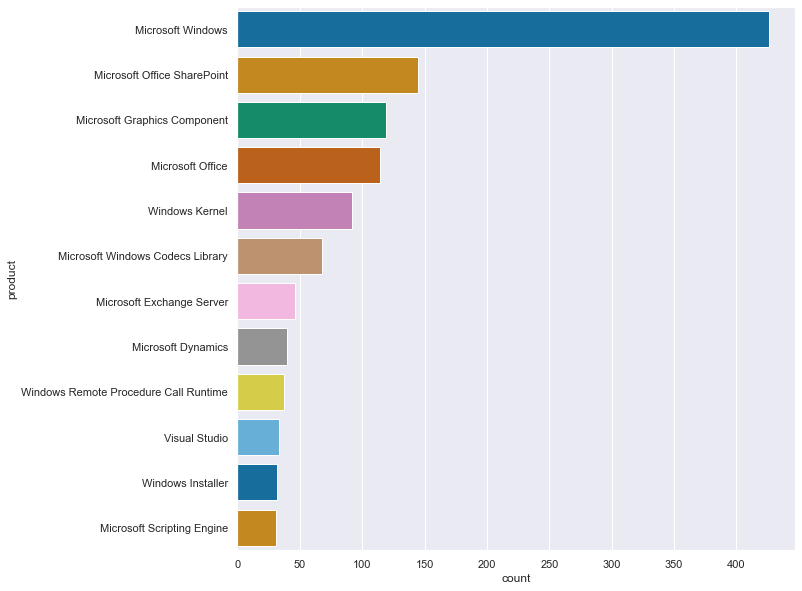
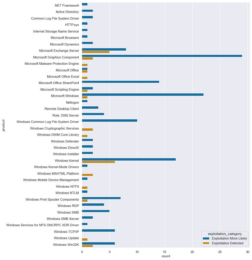
List of most common products in the data, see below for full list.
Limitations
In order to be able to do over- and undersampling with the product field I had to do one-hot encoding on the data. Because the classification was then done on the encoded fields, the coefficients of the model is calculated on these synthetic columns. OneHotEncoder does include an inverse_transform but it would transform an encoded row back to its original - and the calculated coefficients are floating point numbers which do not correspond to actual encoder produced values.
Thus I am, at least with my current knowledge, unable to produce a weighted list of products to look out for. But what I can show is a simple list of products with the more severe categories:
Next steps
The results of this brief study will be summarized with guidance on how IT administrators and other responsible personnel are able to easily integrate Microsoft’s exploitation assessment in their patching routine.
Further research
Ideas for expanding this brief study:
- Add a temporal element: full disclosure / 0day vulns are worse than things that were exploited a year later
- Add more vendors to the mix, or run the same thing on another vendor in isolation
- Expand the time frame from two years as far backwards as the other datasources support
- Map the CVE numbers to branded vulnerabilities to find proof of exploit codes
Appendix
Data sources
- CISA Catalogue of Known Exploited Vulnerabilities
- CVE Details > Microsoft
- Microsoft vulnerabilities
- NCSC-FI Vulnerabilities
- NCSC-FI Alerts
- NCSC-FI News digest
- NCSC-FI Vulnerability digest
- Exploit-db
- Branded vulnerabilities
Learning sources
pandasscikit-learnseaborn- SMOTE for Imbalanced Classification with Python
- How to Use ROC Curves and Precision-Recall Curves for Classification in Python
- Python Data Science Handbook by Jake VanderPlas
- University of Helsinki > Introduction to Data Science
Full list of products
| Product as given in Microsoft vuln API JSON | Count |
|---|---|
| .NET Core | 3 |
| .NET Core & Visual Studio | 5 |
| .NET Framework | 3 |
| .NET Repository | 1 |
| 3D Viewer | 5 |
| ASP.NET | 4 |
| ASP.NET Core & Visual Studio | 2 |
| ASP.NET core & .NET core | 1 |
| Active Directory | 5 |
| Active Directory Federation Services | 3 |
| Android App | 3 |
| Application Virtualization | 1 |
| Apps | 3 |
| Azure | 8 |
| Azure AD Web Sign-in | 1 |
| Azure Active Directory Pod Identity | 1 |
| Azure Bot Framework SDK | 1 |
| Azure DevOps | 11 |
| Azure Open Management Infrastructure | 4 |
| Azure RTOS | 6 |
| Azure SDK | 1 |
| Azure Sphere | 26 |
| BizTalk ESB Toolkit | 1 |
| Common Internet File System | 1 |
| Common Log File System Driver | 5 |
| Console Window Host | 1 |
| Developer Tools | 2 |
| Diagnostics Hub | 3 |
| Dynamics Business Central Control | 2 |
| Group Policy | 1 |
| HTTP.sys | 2 |
| HoloLens | 1 |
| Internet Explorer | 1 |
| Internet Storage Name Service | 1 |
| Jet Red and Access Connectivity | 1 |
| Microsoft Accessibility Insights for Android | 1 |
| Microsoft Accessibility Insights for Web | 1 |
| Microsoft ActiveX | 1 |
| Microsoft Azure Active Directory Connect | 1 |
| Microsoft Azure Kubernetes Service | 1 |
| Microsoft Bing | 1 |
| Microsoft Bluetooth Driver | 4 |
| Microsoft Browsers | 3 |
| Microsoft DTV-DVD Video Decoder | 1 |
| Microsoft Defender for IoT | 10 |
| Microsoft Dynamics | 40 |
| Microsoft Dynamics Finance & Operations | 1 |
| Microsoft Edge (Chromium-based) | 10 |
| Microsoft Edge (HTML-based) | 2 |
| Microsoft Edge for Android | 1 |
| Microsoft Edge for iOS | 1 |
| Microsoft Edge on Chromium | 1 |
| Microsoft Exchange Server | 46 |
| Microsoft Graphics Component | 119 |
| Microsoft Internet Messaging API | 1 |
| Microsoft Intune | 2 |
| Microsoft JET Database Engine | 25 |
| Microsoft Local Security Authority Server (lsasrv) | 1 |
| Microsoft MPEG-2 Video Extension | 1 |
| Microsoft Malware Protection Engine | 5 |
| Microsoft Message Queuing | 2 |
| Microsoft NTFS | 4 |
| Microsoft Office | 114 |
| Microsoft Office Access | 3 |
| Microsoft Office Excel | 30 |
| Microsoft Office Outlook | 2 |
| Microsoft Office PowerPoint | 1 |
| Microsoft Office SharePoint | 145 |
| Microsoft Office Visio | 5 |
| Microsoft Office Word | 6 |
| Microsoft OneDrive | 4 |
| Microsoft PowerShell | 1 |
| Microsoft Scripting Engine | 31 |
| Microsoft Teams | 2 |
| Microsoft Video Control | 1 |
| Microsoft Windows | 426 |
| Microsoft Windows Codecs Library | 68 |
| Microsoft Windows DNS | 11 |
| Microsoft Windows IrDA | 1 |
| Microsoft Windows Media Foundation | 3 |
| Microsoft Windows PDF | 1 |
| Microsoft Windows Search Component | 13 |
| Microsoft Windows Speech | 3 |
| Netlogon | 1 |
| Office Developer Platform | 1 |
| Open Source Software | 6 |
| OpenEnclave | 1 |
| Paint 3D | 3 |
| Power BI | 4 |
| PowerShellGet | 1 |
| Remote Desktop Client | 4 |
| Remote Desktop Connection Manager | 1 |
| Rich Text Edit Control | 1 |
| Role: DNS Server | 19 |
| Role: Hyper-V | 6 |
| Role: Windows AD FS Server | 1 |
| Role: Windows Active Directory Server | 1 |
| Role: Windows Fax Service | 3 |
| Role: Windows Hyper-V | 11 |
| SQL Server | 4 |
| Secure Boot | 1 |
| Skype for Business | 3 |
| Skype for Business and Microsoft Lync | 2 |
| SysInternals | 1 |
| System Center | 3 |
| Visual Studio | 33 |
| Visual Studio Code | 21 |
| Visual Studio Code - .NET Runtime | 1 |
| Visual Studio Code - GitHub Pull Requests and Issues Extension | 1 |
| Visual Studio Code - Kubernetes Tools | 2 |
| Visual Studio Code - Maven for Java Extension | 1 |
| Visual Studio Code - WSL Extension | 1 |
| Windows AF_UNIX Socket Provider | 1 |
| Windows AI | 3 |
| Windows Active Directory | 5 |
| Windows Address Book | 2 |
| Windows Admin Center | 1 |
| Windows Ancillary Function Driver for WinSock | 2 |
| Windows AppContainer | 3 |
| Windows AppX Deployment Extensions | 4 |
| Windows AppX Deployment Service | 1 |
| Windows Application Compatibility Cache | 1 |
| Windows Authentication Methods | 1 |
| Windows Authenticode | 2 |
| Windows Backup Engine | 8 |
| Windows Bind Filter Driver | 3 |
| Windows BitLocker | 1 |
| Windows Bluetooth Service | 1 |
| Windows COM | 7 |
| Windows CSC Service | 8 |
| Windows Cloud Files Mini Filter Driver | 2 |
| Windows Common Log File System Driver | 11 |
| Windows Console Driver | 4 |
| Windows Container Execution Agent | 2 |
| Windows Container Isolation FS Filter Driver | 1 |
| Windows Container Manager Service | 5 |
| Windows Core Shell | 1 |
| Windows Cred SSProvider Protocol | 1 |
| Windows CryptoAPI | 1 |
| Windows Cryptographic Services | 2 |
| Windows DCOM Server | 1 |
| Windows DHCP Server | 1 |
| Windows DP API | 1 |
| Windows DWM Core Library | 2 |
| Windows Defender | 12 |
| Windows Desktop Bridge | 4 |
| Windows Diagnostic Hub | 11 |
| Windows Digital TV Tuner | 1 |
| Windows DirectX | 4 |
| Windows Drivers | 1 |
| Windows ELAM | 1 |
| Windows Early Launch Antimalware Driver | 1 |
| Windows Encrypting File System (EFS) | 2 |
| Windows Error Reporting | 4 |
| Windows Event Logging Service | 2 |
| Windows Event Tracing | 17 |
| Windows Extensible Firmware Interface | 1 |
| Windows Fastfat Driver | 3 |
| Windows Feedback Hub | 1 |
| Windows File History Service | 1 |
| Windows Filter Manager | 1 |
| Windows Folder Redirection | 1 |
| Windows HTML Platform | 2 |
| Windows Hello | 2 |
| Windows Hyper-V | 23 |
| Windows IIS | 1 |
| Windows Installer | 32 |
| Windows Kerberos | 1 |
| Windows Kernel | 92 |
| Windows Kernel-Mode Drivers | 1 |
| Windows Key Distribution Center | 1 |
| Windows Key Storage Provider | 1 |
| Windows Local Security Authority Subsystem Service | 2 |
| Windows Lock Screen | 2 |
| Windows MSHTML Platform | 6 |
| Windows Media | 22 |
| Windows Media Player | 7 |
| Windows Mobile Device Management | 2 |
| Windows NDIS | 2 |
| Windows NTFS | 9 |
| Windows NTLM | 3 |
| Windows Nearby Sharing | 1 |
| Windows Network Address Translation (NAT) | 1 |
| Windows Network File System | 5 |
| Windows OLE | 3 |
| Windows Overlay Filter | 3 |
| Windows PFX Encryption | 2 |
| Windows PKU2U | 1 |
| Windows Partition Management Driver | 1 |
| Windows Portmapping | 1 |
| Windows PowerShell | 1 |
| Windows Print Spooler Components | 20 |
| Windows Projected File System | 1 |
| Windows Projected File System FS Filter | 1 |
| Windows Projected File System Filter Driver | 4 |
| Windows RDP | 14 |
| Windows RDP Client | 1 |
| Windows Redirected Drive Buffering | 4 |
| Windows Registry | 4 |
| Windows Remote Access API | 1 |
| Windows Remote Access Connection Manager | 8 |
| Windows Remote Assistance | 1 |
| Windows Remote Desktop | 3 |
| Windows Remote Procedure Call | 2 |
| Windows Remote Procedure Call Runtime | 37 |
| Windows Resource Manager | 1 |
| Windows SMB | 11 |
| Windows SMB Server | 2 |
| Windows SSDP Service | 1 |
| Windows Scripting | 3 |
| Windows Secure Kernel Mode | 3 |
| Windows Security Account Manager | 1 |
| Windows Services and Controller App | 1 |
| Windows Services for NFS ONCRPC XDR Driver | 5 |
| Windows Shell | 14 |
| Windows Storage | 2 |
| Windows Storage Spaces Controller | 14 |
| Windows Subsystem for Linux | 4 |
| Windows SymCrypt | 1 |
| Windows TCP/IP | 13 |
| Windows TDX.sys | 1 |
| Windows TPM Device Driver | 1 |
| Windows Task Scheduler | 1 |
| Windows Text Shaping | 1 |
| Windows Trust Verification API | 1 |
| Windows UPnP Device Host | 1 |
| Windows Update | 2 |
| Windows Update Assistant | 5 |
| Windows Update Stack | 27 |
| Windows User Profile Service | 4 |
| Windows Virtual Machine Bus | 1 |
| Windows WLAN Auto Config Service | 2 |
| Windows WLAN Service | 1 |
| Windows WalletService | 18 |
| Windows Win32K | 11 |
| Windows Wireless Networking | 1 |
| Windows exFAT File System | 1 |
| Windows splwow64 | 1 |